


Useful Queries (Analytic Cookbook)
Kusto Query Language (KQL) recipes to cook up productive searches.
This page presents KQL analytic search queries that are useful for various specific purposes. Entries describe how the queries work, and show sample results.
Search DDSS Bucket Time Ranges
You can use this query to return DDSS buckets’ time ranges, formatted and sorted:
.show objects(<bucket name>)
| extend  path3=split(name,"/",2) | extend dbpath=split(path3,"_") | extend starttime_epoch=dbpath[1], endtime_epoch=dbpath[2]
| extend starttime=format_datetime(starttime_epoch, 'yy-MM-dd hh:mm:ss tt'), endtime=format_datetime(endtime_epoch, 'yy-MM-dd hh:mm:ss tt')
| project name, size, starttime, endtime
| sort by starttime ascZ-Score-Based Anomaly Detection
This analytic takes a time series Dataset, applies a mean and standard deviation to it, then computes a high-and-low envelope based on mean +/ n*stdev, where N is called the “Z-score.” This is what is commonly referred to as “N standard deviations above/below the average.”
dataset="cribl_edge_metrics" cribl_fleet="default_fleet" host="ip-172-31-91-42.ec2.internal" metrics_source="cpu" node_cpu_percent_active_all
| timestats span=10m cpu_max=max(node_cpu_percent_active_all), cpu_avg=avg(node_cpu_percent_active_all) cpu_stdev=stdev(node_cpu_percent_active_all)  // fetch active cpu statistics (max, mean, stddev)
| extend z_score=4, delta=cpu_stdev*z_score // create a variable z-score, and a delta that represents the z-score times the mean
| extend env_hi=cpu_avg+delta, env_lo=cpu_avg-delta // create an envelope above and below the mean using the delta
| extend env_hi=min_of(env_hi,95), env_hi=max_of(env_hi,5) // fudge factor for the high limit to be within 5% -> 95%
| extend env_lo=max_of(env_lo,1)  // fudge factor for the low limit to be at least 1%
| extend anomaly_flag=iif(cpu_max>env_hi , 1,0), anomaly_chart = cpu_max * anomaly_flag, cpu_max=cpu_max*(1-anomaly_flag) // create a new data series to visualize the anomalies in different color
| project-away z_score, delta, cpu_stdev, cpu_avg // remove the intermediate computation fields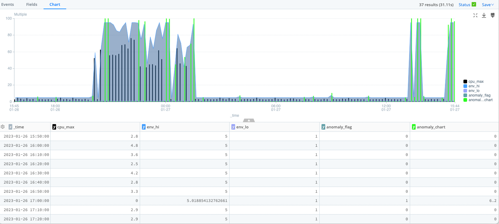
Notes on Z-Score Detection
The various extend operators compute the z-score envelope (env_hi and env_lo) and then compute an anomaly_flag if the actual Dataset (here, cpu_max) is greater than the high envelope.
We use anomaly_chart to visually display the anomalies (points higher than env_hi) in a separate color, highlighting them. (This is a bit of a kludge, since we can’t currently repaint individual data points in a series).
AWS Inventory by Datatype, Objects, Events, TotalBytes
This analytic looks in your S3-based Dataset and counts the number of objects (files, usually), the number of events in those files, and the number of bytes in those events. You can run this over a large sample of data - say, several days - to get a feel for how much data is in your S3 bucket.
The Unsampled Version
This version is expensive, in terms of time and CPU*seconds. Compare it to the sampled version below.
dataset="cribl_search_sample"
| extend eventBytes=strlen(_raw)
| summarize NumEvents=count(), NumObjects=dcount(source), totalBytes=sum(eventBytes) by datatype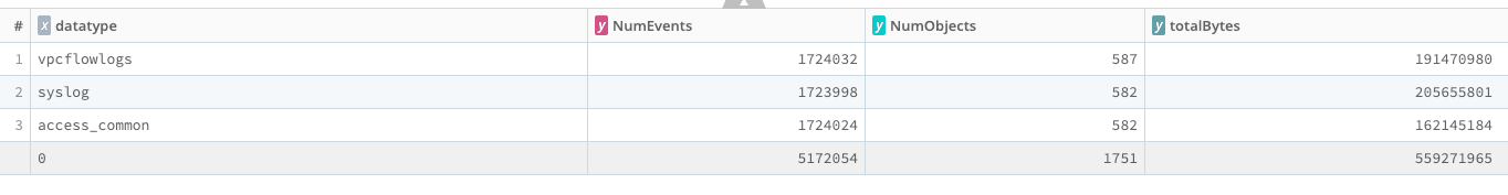

Note: This search took almost 4 minutes of wall clock time and over 11,000 CPU*Seconds to run, equivalent to more than three Cribl credits.
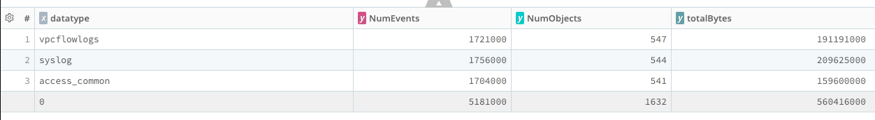
The Sampled Version
The sampled version, run at 1:1000 sampling. (Use this one!) Byte and Event counts are corrected for the sampling error.
dataset="cribl_search_sample"
| extend eventBytes=strlen(_raw)
| summarize NumEvents=count(), NumObjects=dcount(source), totalBytes=sum(eventBytes) by datatype
| extend NumEvents=NumEvents*1000, totalBytes=totalBytes*1000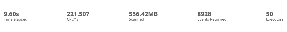
Notes on AWS Optimization
This search took less than 10 seconds of wall clock time to run, and about 220 CPU*seconds, equivalent to only 0.06 Cribl credits.
When run over a large time range (say, 1 day), the sampled version is almost as accurate as the unsampled version (within two or three significant figures). It runs about 25x faster, and costs about 50x less in terms of CPU*seconds.
AWS Cost and Usage Report (CUR) - Parquet Analysis
This analytic is tricky only because the CUR is in Parquet format, and doesn’t have _time in each event. Instead, there’s a field called identity_time_interval, which inexplicably has two timestamps, with a slash separating them. By using a regex to extract them, we can then use one (here, the intervalstarttime) to cast back into _time, and then events will behave as desired.
dataset="billing"
| extract source=identity_time_interval type=regex regex=@"(?<intervalstarttime>.+)\/(?<intervalendtime>.+)"
| extend intervalstarttime=todatetime(intervalstarttime), intervalendtime=todatetime(intervalendtime)
| extend _time=intervalstarttime
| timestats span=1h totalusage=sum(line_item_usage_amount) by product_groupThis particular analytic simply summarizes line_item_usage_amount by product_group, but once the data has been properly formatted, any further analytics are fairly straightforward.
Internal Search Utilization
You can use this search to obtain a more granular view of your own Cribl Search usage.
dataset="cribl_internal_logs" message="search finished"
| summarize sum(stats.cpuMetrics.totalCPUSeconds) by stats.userNote that this example is split by user, but you can change it to split by anything, or eliminate the split by entirely.
Correct for dollars:
dataset="cribl_internal_logs" message="search finished"
| extend totalCost=stats.cpuMetrics.totalCPUSeconds/3600
| timestats span=1d sum(totalCost) by stats.userDisplayNameJournalD Search via Edge
This search will connect to your Edge fleet and search JournalD files on all hosts in the fleet for Command Line arguments.
dataset="cribl_edge_journal" journald._CMDLINE=*
| limit 100
| project _time,host,journald._CMDLINE,journald._PID,journald._UID,journald._GIDfThis requires that you’ve created a Dataset called cribl_edge_journal, which is of type Edge, and filtered to look at journal files in /var/log. Here’s an example of how to set up the Dataset:
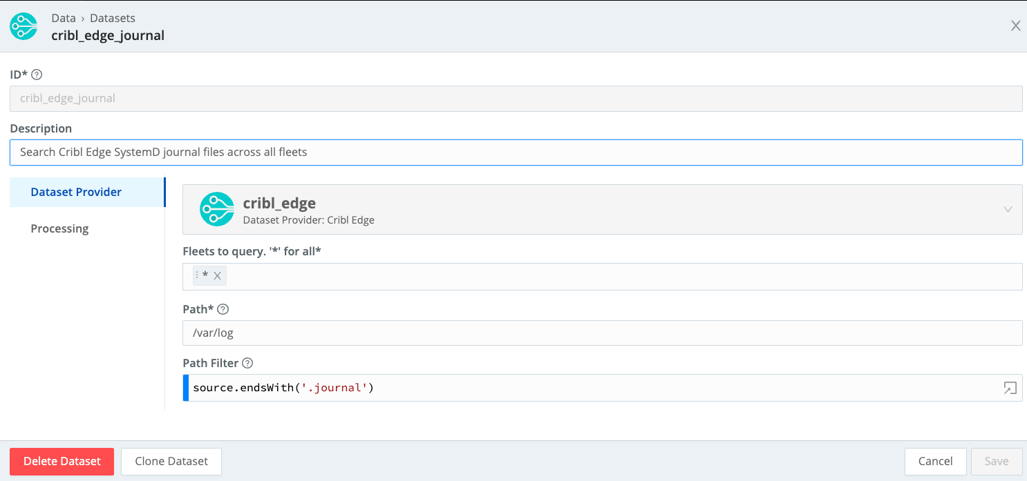
You can query specific Fleets by tailoring the Fleets to query field.
Splunk VPC Flow Logs Search via S3
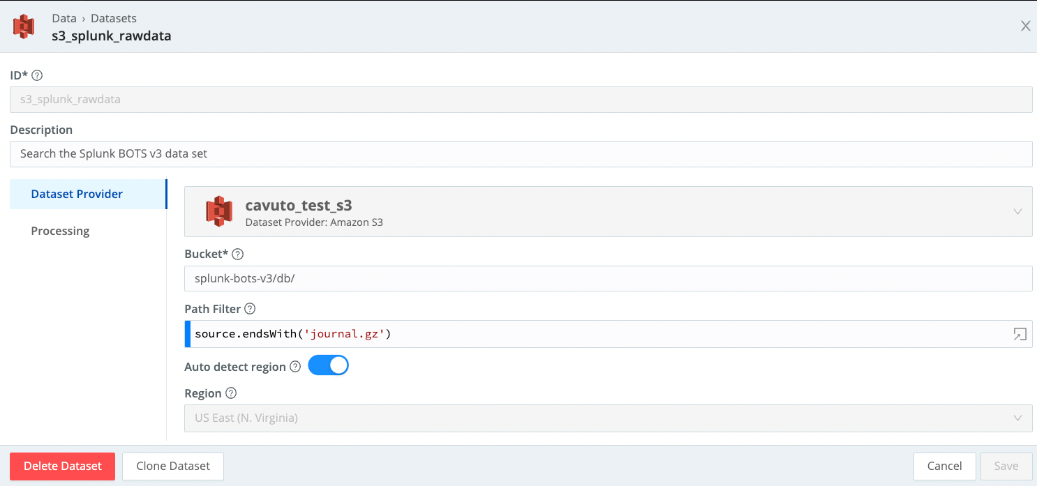
This earches a set of Splunk rawdata (journal.gz) files in a bucket in S3, then extracts the results using an existing parser.
dataset="s3_splunk_rawdata" sourcetype=*vpc*
| limit 1000
| extract parser='AWS VPC Flow Logs'This requires a Dataset pointing to a set of Splunk files. It will descend into subfolders - need not be flat.
All Splunk compression formats are supported, including .zip, .gz, and .lzw.
Search a Data Lake Populated from Cribl Stream
Any specific search will work on this Dataset.
dataset="data_lake" | limit 1000 Partitioning scheme needs to set to:
${}-${_time:%Y}/${}-${_time:%m}/${}-${_time:%d}/${}-${_time:%H}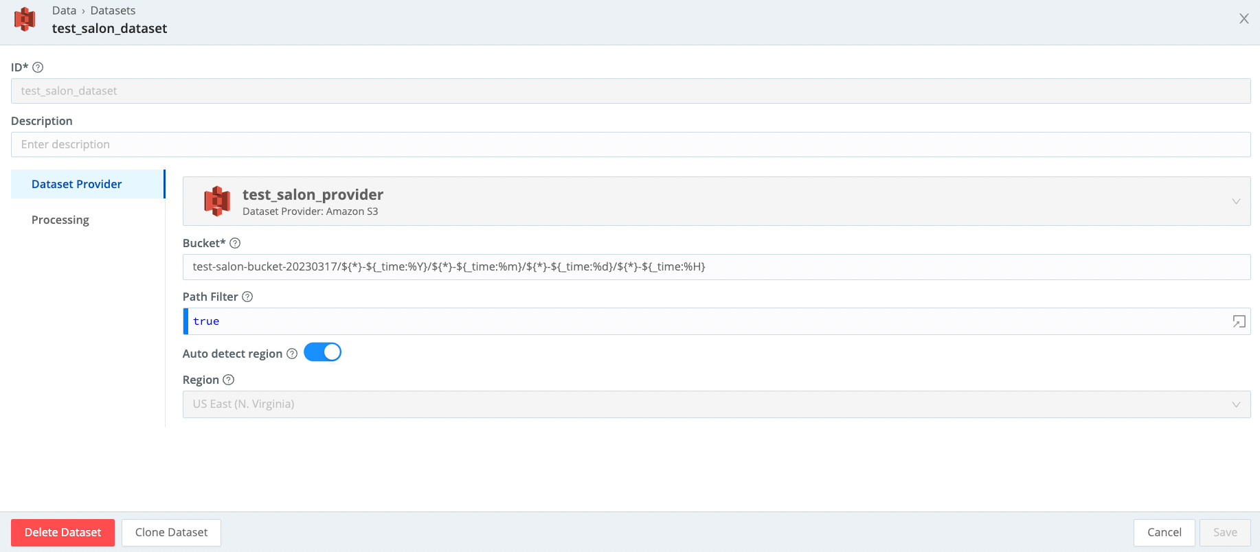
Send Cribl Search Results to Cribl Stream
Enables you to take arbitrary Cribl Search results and send them to Cribl Stream with the send operator.
dataset="s3_splunk_rawdata" sourcetype=*vpc*
| extract parser='AWS VPC Flow Logs'
| where srcaddr in~ ("34.215.24.225", "172.16.0.178") and dstaddr in~ ("172.16.0.178", "34.215.24.225")
| send tee=false group=default This is just an example of how to drill down into a Dataset (here, using the Splunk BOTS Dataset), and then send the results to Stream.
Internal-to-External Network Conversations
This analytic works with BOTS v3 Data:
dataset="bots_v3" sourcetype in ("stream:tcp", "stream:udp")
| limit 1000
| extract type=json
| where isnotnull(src_ip) and isnotnull(dest_ip)
| lookup matchMode='cidr' cidr_1918_blocks on src_ip=cidr_block
| extend src_network_type=network_type
| lookup matchMode='cidr' cidr_1918_blocks on dest_ip=cidr_block
| extend dest_network_type=network_type
| where src_network_type=="private" and dest_network_type=="public"
| summarize values(dest_port), session_count=count() by src_ip, dest_ip This analytic works with VPC Flow Logs:
dataset="cribl_search_sample" dataSource=*vpc* | limit 1000
| where isnotnull(srcaddr) and isnotnull(dstaddr)
| lookup matchMode='cidr' cidr_1918_blocks on srcaddr=cidr_block
| extend src_network_type=network_type
| lookup matchMode='cidr' cidr_1918_blocks on dstaddr=cidr_block
| extend dest_network_type=network_type
| where src_network_type=="private" and dest_network_type=="public"
| summarize values(dstport), session_count=count() by srcaddr, dstaddrRequires creating this lookup table:
cidr_block,network_type
10.0.0.0/8,private
127.0.0.0/8,loopback
172.16.0.0/12,private
192.168.0.0/16,private
0.0.0.0/0,publicDataset Usage Stats
Analyze Cribl Search logs to understand the Datasets with the highest number of searches, number of users who have searched, when the last search was, and what the average search time is. Admins can use this analytic to help discover which Datasets would offer the highest return if optimized.
dataset="cribl_internal_logs" source=="file:///opt/cribl/log/searches.log" stats.status="completed"
 | limit 1000
 | extract source=stats.query @'dataset=\"(?<datasetUsed>\S+)\"'
 | where datasetUsed
 | summarize searchCount = dcount(stats.id), lastSearch = max(_time), users = dcount(stats.user), averageSearchTimeSec = round(avg(stats.elapsedMs)/1000,2) by datasetUsed
 | extend lastSearch = strftime(lastSearch, '%Y-%m-%dT%H:%M:%S.%L%Z')
 | sort by searchCount desc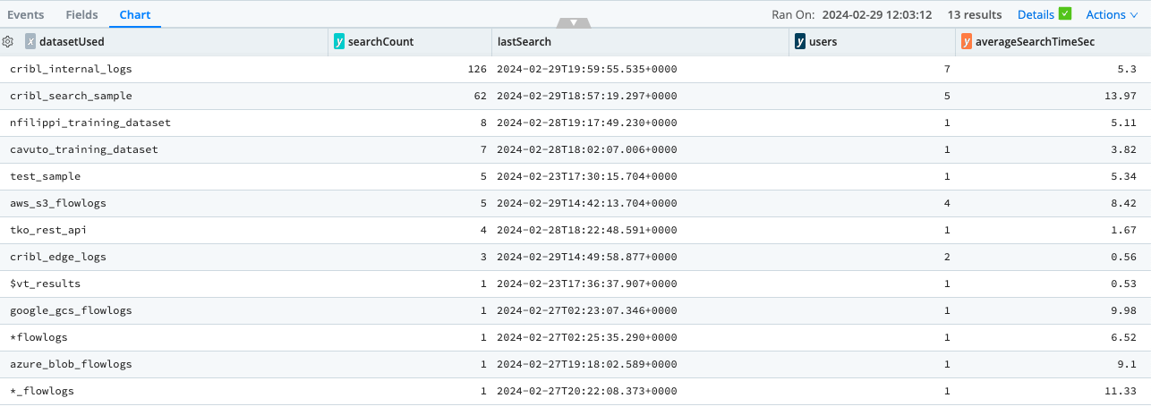
Timerange Distribution
What timerange do users most often use when running ad hoc (standard) searches?
dataset="searches" stats.status in ("completed","failed","canceled") stats.type="standard"
 | extract source=stats.searchTimeRange type=regex @'(?<timeRangeValue>\d*)'
 | extract source=stats.searchTimeRange type=regex @'\d*(?<timeRangeModifier>\D*)'
 | extend timeRangeMultiplier = case (timeRangeModifier == "ms", 0.000000277777778,
                                        timeRangeModifier == "s", 0.000277777778,
                                        timeRangeModifier == "m", 0.01666666666,
                                        timeRangeModifier == "h", 1,
                                        timeRangeModifier == "d", 24,
                                        timeRangeModifier == "M", 730,
                                        timeRangeModifier == "y", 8760,
                                        "none")
 | where timeRangeMultiplier != "none"
 | extend timeRangeHours = round(timeRangeValue * timeRangeMultiplier,2)
 | summarize within_1h=sum(iff(timeRangeHours <= 1,1,0)),
             within_1d=sum(iff(timeRangeHours <= 24,1,0)),
             within_7d=sum(iff(timeRangeHours <= 168,1,0)),
             within_14d=sum(iff(timeRangeHours <= 336,1,0)),
             within_30d=sum(iff(timeRangeHours <= 730,1,0)),
             within_1y=sum(iff(timeRangeHours <= 8760,1,0)),
             total=count()
| project within_1h = strcat(within_1h, ' (', round(within_1h/total*100,2), '%)'),
          within_1d = strcat(within_1d, ' (', round(within_1d/total*100,2), '%)'),
          within_7d = strcat(within_7d, ' (', round(within_7d/total*100,2), '%)'),
          within_14d = strcat(within_14d, ' (', round(within_14d/total*100,2), '%)'),
          within_30d = strcat(within_30d, ' (', round(within_30d/total*100,2), '%)'),
          within_1y = strcat(within_1y, ' (', round(within_1y/total*100,2), '%)'),
          all = strcat(total, ' (', round(within_total/total*100,2), '%)')