/ / / /

Sizing and Scaling

A Cribl Stream installation can be scaled up within a single instance and/or scaled out across multiple instances. Scaling allows for:

Increased data volumes of any size.
Increased processing complexity.
Increased deployment availability.
Increased number of destinations.

We offer specific examples below, and introduce reference architectures in Architectural Considerations.

Scale Up

A Cribl Stream deployment can be configured to scale up and utilize as many resources on hosts as required. You control this differently on Cribl-managed versus customer-managed Worker Groups.

To optimize Cribl-managed Worker Nodes in Cribl.Cloud, navigate to the desired Worker Group’s Group Settings > Group Configuration section. Then adjust the Sizing Calculator to determine the appropriate size for your Worker Group.

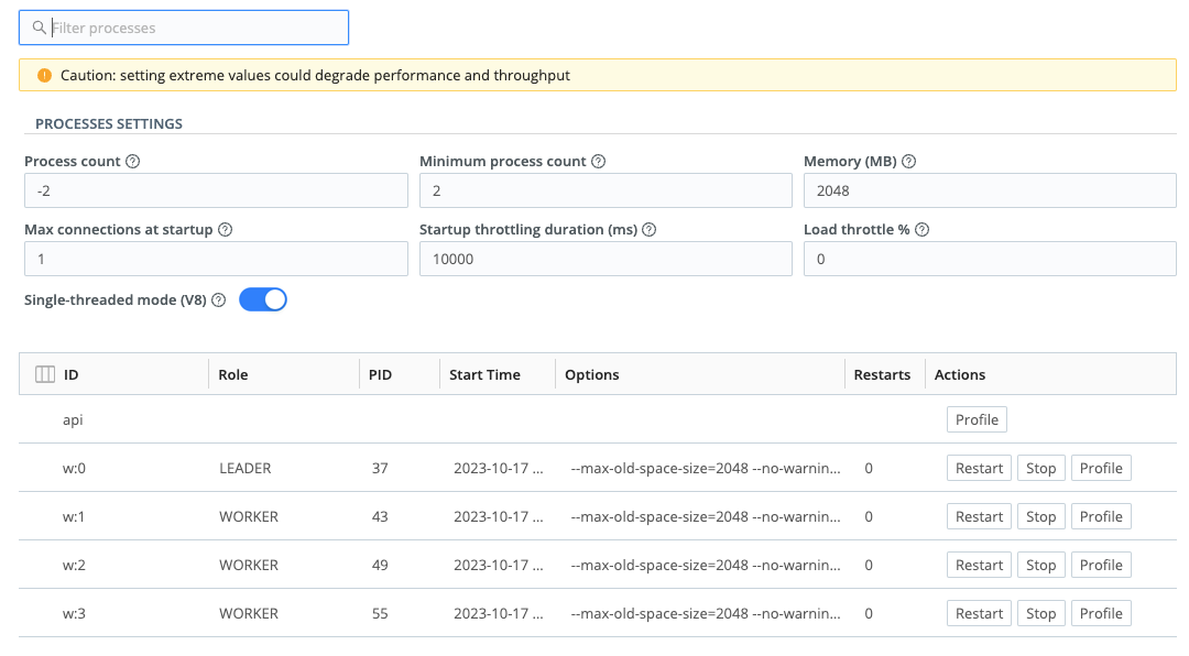
With an on-prem Single-instance deployment, you govern resource allocation in Settings > System > Service Processes > Processes section.

With an on-prem Distributed deployment or hybrid group, you allocate resources per Worker Group. From Stream Home, navigate to Worker Groups > group-name > Group Settings > Worker Processes.

In any of the above on-prem scenarios, these controls are available:

Process count: Indicates the number of Worker Processes to spawn. Positive numbers specify an absolute number of Workers. Negative numbers specify a number of Workers relative to the number of CPUs in the system, for example: {<number of CPUs available> minus <this setting>}. The default is -2.
Cribl Stream will correct for an excessive + or - offset, or a 0 entry, or an empty field. Here, it will guarantee at least the Minimum process count set below, but no more than the host’s number of CPUs available.
Minimum process count: Indicates the minimum number of Worker Processes to spawn. Overrides the Process count’s lowest result. A 0 entry is interpreted as “default,” which here yields 2 Processes.
Memory (MB): Amount of heap memory available to each Worker Process, in MB. Defaults to 2048 (see Estimating Memory Requirements). Heap memory is allocated dynamically from the OS as it is requested by the Process up to the amount dictated by this setting. The Memory (MB) setting does not govern external (ext) memory.
If a Process needs more than the allocated amount of heap memory, it will encounter an Out of memory error, which is logged to $CRIBL_HOME/log/cribl_stderr.log. This error indicates either:
- A memory leak.
- The memory setting is too low for the workload being performed by the Process (and possibly, by extension, that the total memory provisioned for the host is insufficient for all Processes).
Cribl support can help you troubleshoot if you experience this error.

For changes in any of the above controls to take effect, you must select Save and then restart the Cribl Stream server via Settings > Global > System > Controls > Restart. In a distributed deployment, also deploy your changes to the Groups.

For example, assuming a Cribl Stream system running on Intel or AMD processors with 6 physical cores hyperthreaded (12 vCPUs):

If Process count is set to 4, then the system will spawn exactly 4 processes.
If Process count is set to -2, then the system will spawn 10 processes (12-2).

Allocate a Maximum Number of Worker Processes

To provision a container with a set number of Worker Processes, use the CRIBL_MAX_WORKERS environment variable.

Worker processes handle data ingestion and processing tasks. Improper configuration can lead to:

Unstable container deployments: Incorrect Worker Process settings might cause your containers to malfunction or become unstable.
Outages: Unforeseen resource consumption due to excessive number of Worker Processes can lead to Cribl crashing and service outages.

A couple notes about the CRIBL_MAX_WORKERS environment variable:

The value you designate represents the maximum number of Worker Processes for the container. If there are fewer actual CPUs than designated in the variable, the container will provision with the number of Worker Processes that match the actual number of CPUs.
Several different factors determine the final number of Worker Processes. Cribl uses the lowest number of all of these:
- The Cribl license Worker Process limit
- The number of actual Worker Processes (with Process count factored in)
- The Worker count configured in cribl.yml
- CRIBL_MAX_WORKERS (if configured)
For example:
- License limit: 7
- Number of actual Worker Processes (OS based): 4, calculated as number of actual Worker Processes (6) and Process count (-2)
- Worker Processes in cribl.yml: 5
- CRIBL_MAX_WORKERS: 3
There are three final assigned Worker Processes, because 3 is the lowest number of all the values above.

Example configurations

Docker

docker run -e CRIBL_MAX_WORKERS=2

Helm

helm install --set env.CRIBL_MAX_WORKERS=2

The values.yml file

env:
  CRIBL_MAX_WORKERS: 2

By default, Cribl sets the Worker Process count to -2 (Worker Processes (CPU cores) = total CPU cores - 2 ). If you don’t configure CRIBL_MAX_WORKERS and directly launch a container, it inherits the default behavior. This can lead to inefficient resource usage, particularly on machines with many CPU cores.

Scale Out

When data volume, processing needs, or other requirements exceed what a single instance can sustain, a Cribl Stream deployment can span multiple Nodes. This is known as a distributed deployment. Here, you can centrally configure and manage Nodes’ operation using one administrator instance, called the Leader.

It’s important to understand that Worker Processes operate in parallel, i.e., independently of each other. This means that:

Data coming in on a single connection will be handled by a single Worker Process. To get the full benefits of multiple Worker Processes, data should come in over multiple connections.
For example, it’s better to have five connections to TCP 514, each bringing in 200GB/day, than one at 1 TB/day.
Each Worker Process will maintain and manage its own outputs. For example, if an instance with two Worker Processes is configured with a Splunk output, then the Splunk destination will see two inbound connections.
For further details, see Shared-Nothing Architecture.

Capacity and Performance Considerations

As with most data processing applications, Cribl Stream’s expected resource utilization will be proportional to the type of processing that is occurring. For instance, a Function that adds a static field on an event will likely perform faster than one that applies a regex to find and replace a string. Currently:

A Worker Process will utilize up to 1 physical core (encompassing either 1 or 2 vCPUs, depending on the processor type.
Processing performance is proportional to CPU clock speed.
All processing happens in-memory.
Processing does not require significant disk allocation.

Throughout these guidelines, we assume that 1 physical core is equivalent to:

2 virtual/hyperthreaded CPUs (vCPUs) on Intel/Xeon or AMD processors.
1 vCPU on Graviton2/ARM64 processors.

Overall guideline: Allocate 1 physical core for each 400GB/day of IN+OUT throughput.

Examples

Estimating Number of Cores

In estimating core requirements – per processor type, it’s important to distinguish among vCPUs versus physical cores.

Intel/Xeon/AMD Processors with Hyperthreading Enabled

To estimate the number of cores needed: Sum your expected input and output volume, then divide by 400GB per day per physical core.

Example 1: 100GB IN ‑> 100GB out to each of 3 destinations = 400GB total = 1 physical core (or 2 vCPUs).
Example 2: 3TB IN ‑> 1TB out = 4TB total = 10 physical cores (or 20 VCPUs).
Example 3: 4 TB IN ‑> full 4TB to Destination A, plus 2 TB to Destination B = 10TB total = 25 physical cores (or 50 vCPUs).

Graviton2/ARM64 Processors

Here, 1 physical core = 1 vCPU, but overall throughput is ~20% higher than a corresponding Intel or AMD vCPU. So, to estimate the number of cores needed: Sum your expected input and output volume, then divide by 480GB per day per vCPU.

Example 1: 100GB IN -> 100GB OUT to each of 3 destinations = 400GB total = 1 physical core.
Example 2: 3TB IN -> 1TB OUT = 4TB total = 8 physical cores.
Example 3: 4 TB IN -> full 4TB OUT to Destination A, plus 2 TB OUT to Destination B = 10TB total = 21 physical cores.

Remember to also account for an additional core per Worker Node for OS/system overhead.

Estimating Number of Nodes

When sizing the number of Stream Worker Nodes, there are two other factors to consider:

Number of Nodes sized for peak workloads;
Number of Nodes offline.

This will allow you to create a robust Cribl Stream environment that can handle peak workloads even during rolling restarts and maintenance downtime.

General guidance includes:

On each Node, Cribl recommends at least 4 ARM vCPUs, or at least 8 x86 vCPUs (i.e., 4 cores with hyperthreading). Below this theshold, the OS overhead from reserved threads claims an excessive percentage of your capacity.
On each Node, Cribl recommends no more than 48 ARM vCPUs, or 48 x86 vCPUs (i.e., 24 cores with hyperthreading). This allocation handles disk I/O requirements when persistent queueing engages.
Plan to successfully handle peak workloads even when 20% of your Worker Nodes are down. This allows for OS patching, and for conducting rolling Stream upgrades and restarts.
For customers in the 5–20 TB range, size for 4‑8 Worker Nodes per Worker Group.

Sizing Example for a Deployment

Step 1: Calculate the total inbound + outbound volume for a given deployment.

In this example, your deployment has 6TB/day streaming into Worker Nodes for a given site, and this data is being routed to both cheap mass storage (S3) and to your system of analysis – 10 TB/day going out.

Stream Workers must have enough CPUs to handle a total of 16 TB per day IN+OUT.

Step 2: From the available server configurations, size the correct number of Nodes for your environment.

You are considering an AWS Compute-optimized Graviton EC2 instance, with either 16-vCPU or 8-vCPU options. We’ll walk you through how to calculate based on each option.

Using Graviton 16-vCPU instances

Each Node would have 15 vCPUs available to Cribl Stream, each at 480 GB per day per vCPU.
15 vCPUs per Node at 480 GB per day per CPU = 7200 GB/day per Node.
7200 GB/day divided by 1024 GB/TB = 7 TB/day.
To handle the workload of 16 TB/day, you need 3 Nodes. Make sure you always round up.
20% of 3 Nodes ≈ 1 Node. Make sure you always round up. To provide for redundancy during patching, maintenance, or restarts, you need one additional server.

With 4x 16-vCPU Nodes, you have 28 TB/day capacity, and can support 21 TB/day with one Node down.

Using Graviton 8-vCPU instances

Each Node would have 7 vCPUs available to Stream, each at 480 GB per day per vCPU.
7 vCPUs per Node at 480 GB per day per CPU = 3360 GB/day per Node.
3360 GB/day divided by 1024 GB/TB = 3.3 TB/day.
To handle the workload of 16 TB/day, you need 5 Nodes. Make sure you always round up.
20% of 5 Nodes = 1 Node. To provide for redundancy during patching, maintenance, or restarts, you need one additional server.

With 6x8‑vCPU Nodes, you have 19.8 TB/day capacity, and can support 16.5 TB/day with one Node down.

If you are optimizing for price, AWS pricing is linear based on the total number of cores. So six 8‑vCPU systems are roughly 75% the cost of four 16-vCPU systems.

If you are optimizing for potential future expansion, the 4x16-vCPU systems would offer ideal additional capacity.

Estimating Memory Requirements

It can be difficult to determine how much heap memory you need, although we do have specific guidance for large lookups. In general, we recommend that you start with the default heap memory allocation of 2048 MB (2 GB) per Worker Process, and add more memory as you find that you’re hitting limits.

Heap memory use is consumed per component, per Worker Process, as follows:

Lookups are loaded into heap memory. Large lookups require extra heap memory allocation (see Memory Sizing for Large Lookups).
Stateful Functions (Aggregations and Suppress) consume heap memory proportional to the rate of data throughput.
The Aggregations Function’s consumption of heap memory further increases with the number of Group by fields.
The Suppress Function’s consumption of heap memory further increases with the cardinality of events matching the Key expression. A higher rate of distinct event values will consume more heap memory.

External Memory

External memory is allocated to in-memory buffers to hold data to be delivered to downstream services. Downstream services can consume as much external memory as they need, up to the limit that the operating system has available. External memory is not subject to the heap memory limit that you can configure in Cribl.

Destinations are the main consumers of external memory. It can be difficult to determine how much external memory you need, although file-based Destinations require more in-memory buffers and therefore more external memory. In a load-balanced configuration, the amount of external memory that a Destination consumes increases with the number of configured endpoints. For example, Splunk Load Balanced (LB) Destinations may use up to 4 MB of memory for each indexer, which means that a single Splunk LB Destination with 300 indexers could require 1.2 GB of extended memory per process.

Recommended AWS, Azure, and GCP Instance Types

Meet sizing requirements with multiples of the following instances. In all cases, reserve at least 5GB disk storage per instance, and more if you enable persistent queuing.

AWS

For Amazon EC2 compute optimized instances. For other options, see the AWS documentation.

Architecture	Minimum	Recommended
Intel	c5d.2xlarge (4 physical cores, 8vCPUs) c5.2xlarge (4 physical cores, 8vCPUs)	c5d.4xlarge or higher (8 physical cores, 16vCPUs) c5.4xlarge or higher (8 physical cores, 16vCPUs)
Graviton2/ARM64	c6g.2xlarge (8 physical cores, 8vCPUs) c6gd.2xlarge (8 physical cores, 8vCPUs)	c6g.4xlarge or higher (16 physical cores, 16vCPUs) c6gd.4xlarge or higher (16 physical cores, 16vCPUs)

Azure

Architecture	Minimum	Recommended
Intel (Fsv2 sizes series)	Standard_F8s_v2 (4 physical cores, 8vCPUs)	Standard_F16s_v2 or higher (8 physical cores, 16vCPUs)
Arm (Dplsv5 sizes series)	Standard_D8pls_v5 (8 physical cores, 8vCPUs)	Standard_D16pls_v5 or higher (16 physical cores, 16vCPUs)

GCP

For compute-optimized machine types.

Architecture	Minimum	Recommended
Intel	c2-standard-8 (4 physical cores, 8vCPUs) n2-standard-8 (4 physical cores, 8vCPUs)	c2-standard-16 or higher (8 physical cores, 16vCPUs) n2-standard-16 or higher (8 physical cores, 16vCPUs)

Measuring CPU or API Load

You can profile CPU and API usage on individual Worker Processes.

Single-Instance Deployment

Go to Settings > System > Service Processes > Processes, and select Profile on the desired row.

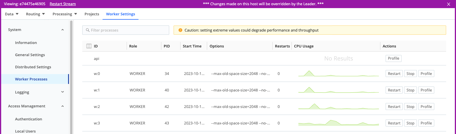
Distributed Deployment

This requires a few more steps:

Enable UI access to Workers if you haven’t already.
In the sidebar, select Workers.
Select the GUID link of the Worker Node you want to profile.
Select Worker Settings from that Worker Node’s submenu.
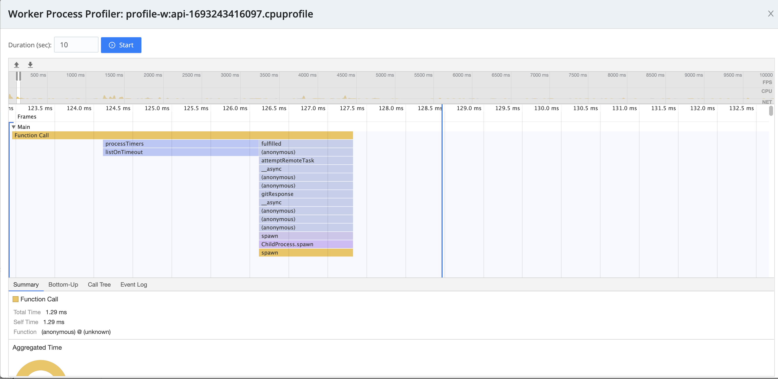
Select System > Worker Processes, and then select Profile on the desired Worker Process. To profile the API usage, click Profile on the api row.

Generating a CPU or API Profile

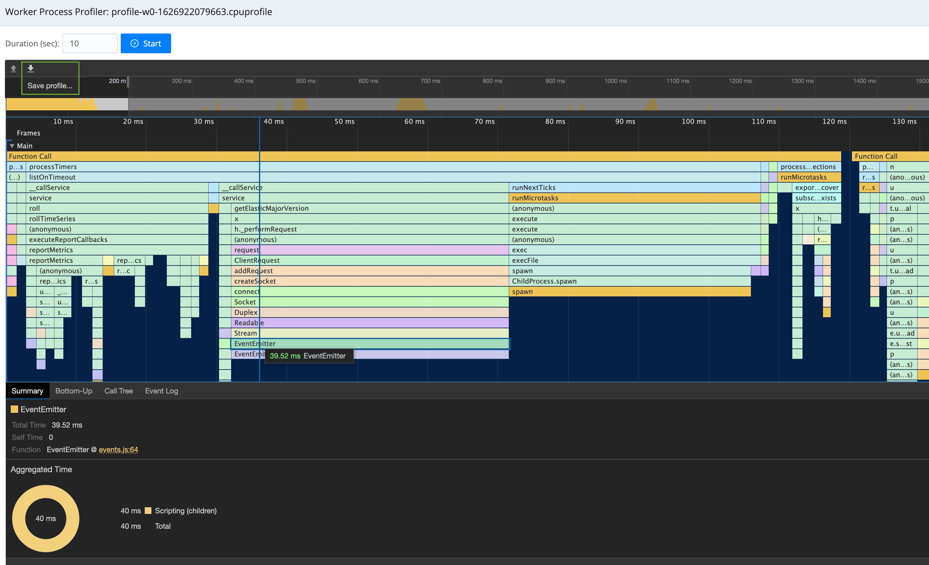
In either a single-instance or distributed deployment, you will now see a Worker Process Profiler modal.

The default Duration (sec) of 10 seconds is typically enough to profile continuous issues, but you might need to adjust this – up to several minutes – to profile intermittent issues. (Longer durations can dramatically increase the lag before Cribl Stream formats and displays the profile data.)

Click Start to begin profiling. After the duration you’ve chosen (watch the progress bar), plus a lag to generate the display, you’ll see a profile something like this:

Worker CPU profile

Profiling the API process can be a helpful troubleshooting tool if the Leader is slow.

API profile

Below the graph, tabs enable you to select among Summary, Bottom‑Up, Call Tree, and Event Log table views.

To save the profile to a JSON file, click the Save profile (⬇︎) button we’ve highlighted at the modal’s upper left.

Whether you’ve saved or not, when you close the modal, you’ll be prompted to confirm discarding the in-memory profile data.

Sizing and Scaling

Scale Up