


Architectural Considerations
This guide introduces Cribl Stream reference architectures by outlining some considerations to keep in mind when architecting your deployment. It covers different potential architectures, with each approach’s advantages, limitations, and alternatives.
Architecting a deployment is always about finding the balance between cost versus risk. Once you’re familiar with the contents of this guide, you’ll be able to consciously make decisions about where your deployment should sit on that spectrum.
See our reference architectures for different use cases. You can replay several Webinar presentations of this material on Cribl’s YouTube channel.
“It Depends”
This guide is not intended to replace Sizing and Scaling, but rather to complement it by outlining the consequences of various architectural decisions. (As needed, please either read Sizing and Scaling first, or refer to it to look up concepts.)
General Sizing Considerations
Some basic sizing variables are your processors, expected data throughput, and requirements for memory, disk space, connections volume, and the Stream Leader’s own needs.
Processors
Your primary consideration in sizing processors is your data throughput capacity, which depends on the number of Worker Processes.
Overall guideline: Allocate 1 physical core for each 400GB/day of IN+OUT throughput.
This can vary based on processor speeds or types. (For example, Graviton ARM processors’ throughput is 20% higher than x86-64 processors’ reference 400GB/day.) But in this guide’s calculations, we’ll assume 400GB/day IN+OUT per processor, and dig into what that really means. Please adjust your own calculations as needed.
Throughput
Where we reference total throughput capacity below: Because Cribl Stream can send events to multiple Destinations and filter out unneeded events, IN won’t always be the same as OUT. For example, 400GB IN+OUT could mean 200GB IN + 200GB OUT, but it could also mean 300GB IN + 100GB OUT, or any combination of IN+OUT that adds up to 400GB/day.
Memory
Memory requirements also play into architecture considerations. Depending on what type of processing you’ll be doing, those requirements might vary. You might know your memory requirements in advance. Or you might monitor memory usage and increase it as your processing complexity increases. The default of 2GB per Worker Process is a good starting point.
Since version 4.13, due to an upgrade of the Node.js version used by Cribl Stream, baseline memory usage may increase on hosts that are not memory-constrained, because the new Node.js version is more conservative with memory release.
Disk Space
The base recommendation, 5GB of free disk space, applies to the volume where Cribl Stream is installed. Beyond that, if you choose to use Persistent Queues, you will need to calculate additional disk space - based on the velocity of your data, and your desired duration before reaching a full queue. Normally, you must define the maximum disk space a queue can use, per Worker Process, for each Source or Destination. However, if you use a separate volume for Persistent Queues, you can remove those limits, and allow the queues to take up the whole volume if needed.
Object-store Destinations use a staging directory to write out files before sending them out. If you’re using one of these Destinations, please review our Amazon S3 Better Practices for sizing and architecture considerations.
In both cases, using fast disks is important, to prevent the disks from becoming bottlenecks.
Number of Connections
Beyond throughput, you have to effectively manage the connection overhead. A single connection limits the workload to one Worker Process. Consider configuring the maximum number of concurrent connections (depending on your Source) to distribute the data and boost the total bytes per process the system handles. When dealing with high-volume streams, use frequent connection rotation (low reuse).
Worker Processes enforce specific concurrent limits on incoming Sources:
TCP Sources (such as Splunk, Syslog, raw TCP): The limit is usually
1,000active connections per Worker Process (WP). Reaching this limit can cause connection failures. You can increase the limit, but be aware that more concurrent activity directly increases the demand on CPU and memory.HTTP-family Sources (such as Cribl HTTP, Splunk HEC, Windows Event Forwarding, OTel HTTP): The limit is usually
256active requests per WP. For HTTP traffic, the number of active requests being processed at any moment is more critical than the total number of open connections. Reaching the limit will result in anHTTP 503 Server is busyresponse.
When you see rejected requests (such as HTTP 503 errors or debug logs showing Dropping request), it indicates you might need to increase the active limit.
Scaling decisions should be based on multiple factors:
- Worker Process limits: The concurrent limits on incoming Sources.
- Bytes-Per-Second (BPS): The objective metric for the workload.
- Connection churn: How often connections are started and stopped (low reuse).
- Data complexity: The impact of your processing Pipeline on resource demand.
- Client limits: The number of parallel connections supported by the sending system (e.g., a single-connection limit on a firewall). Load-balancing features may be necessary to overcome single-connection limits on a client.
Increasing a limit allows more data to be ingested concurrently, which places immediate, higher demands on CPU and memory. You must ensure your infrastructure has sufficient excess capacity to handle the resulting processing load.
The ideal limit depends on your goals and resources. To prevent all rejections (if infrastructure allows), set the limit to 0 (unlimited).
You do not need to worry about “port exhaustion” (running out of available local ports) because many incoming connections can share a single listening port. The system manages these connections efficiently using internal file limits. Monitor these limits and memory usage when you increase the connection cap.
Monitor memory carefully when using TCP Destinations that load balance to many unique targets. The issue isn’t a single Destination configuration, but the total number of target host connections maintained by each Worker Process. Each connection consumes 2 to 4 MB of memory. To manage high memory consumption in these scenarios, set a connection limit (non-zero value) on the load-balancing Destination. You must determine the specific limit based on your available resources.
Leader Node
All the above discussion concerns Worker Nodes, because they are the ones responsible for processing the data. The Leader Node requirements should not need to expand beyond these initial recommendations, unless the Leader needs to manage Edge Fleets, in which case reference Cribl Edge docs.
Finding the Balance Between Risk and Cost
Beyond your basic requirements, you should of course plan contingency capacity to support resource demands that exceed ideal circumstances.
Plan for Failure
Given the wrong circumstances, failure will happen. Your job, when architecting a deployment, is to examine the various failure scenarios and decide what level of resources you are willing to allocate to prevent failure. This is analogous to deciding how many nines of reliability you’re willing to pay for.
Throughput Variability
The 400GB/day IN+OUT guidance mentioned above assumes that your data flow is relatively flat. This means you’re expecting that every second, each Worker Process is handling about ~4.74MB of data IN+OUT. However, in reality, the load varies based on time of day or other system activities.
For example, you might experience higher load during business hours. Or you might have an hourly upstream process that causes spikes of activity. Also, depending on the nature of your organization, you might have certain days, or planned events, when you expect users’ increased load on your systems. Then there are unplanned events, such as outages or DDoS attacks, that might lead to decreased capacity or increased demands.
Another factor to consider, if you’re using Persistent Queues, is that flushing those queues will increase the total throughput demand - including on the downstream systems that need to be able to handle the burst. Unfortunately, there are too many variables to have a generic recommendation here, but a starting point of ~10% headroom is a good idea. As we discuss in the conclusion, you’ll need to test these assumptions.
Now that we’re digging deeper into throughput, you should start thinking about where to set a threshold, beyond which you know your system is likely to fail. If you have data flowing into a system of analysis that can let you look at your current ingestion rate, this can be a good start.
You want to look at the busiest times, and drill down far enough to see what your historical maximum per-second throughput has been. Past performance is not guarantee of future results, but it will at least give you an idea of what to expect.
If you have new Sources, or if you don’t have a good way of estimating current throughput, you’ll have to make some assumptions about future behavior. In the end, take whatever you come up with for expected MB/sec throughput, add whatever safety margin you feel is appropriate, and multiply back out by 84 (24*60*60/1024) to get GB/day throughput.
Exceeding Capacity
As you are deciding how much safety margin to plan into your environment, it also helps to think through what happens when you exceed capacity. Depending on the types of Sources you have, an overloaded deployment might have different failure modes. This ranges from the possibility of immediate data loss in the case of UDP, to simple delays in the case of Pull Sources. Some Push Sources, such as Cribl Edge or Splunk Universal Forwarders, have the capacity to pause or buffer the data flow for some duration.
Separate Data by Worker Groups, Routes, or Both
If you adopt a distributed deployment with multiple Worker Groups, we recommend separating your data volume by Worker Groups, Routes, or a combination of both, depending on your business needs. Common business reasons for sorting by Worker Groups include data isolation by business group, data privacy, and cost savings through geo-isolation. Also, consider which method of separation will be easier to understand and manage as your organization grows.
Connecting Cribl Stream Groups/Instances
When sending data between Workers (whether they report to the same or to different Leaders), use the Cribl HTTP Source and Destination pair, or the Cribl TCP Source and Destination pair. Ingest data usage is only charged to the receiving Organization.
While Cribl Stream supports multiple Sources/Destinations for sending and receiving, TCP JSON is ideal because it supports TLS, has solid compression, and is overall well-formatted to maintain data’s structure between sender and receiver.
Single-Instance Deployment
The simplest type of deployment is single-instance. Let’s look at the case of a 4 core (8 vCPUs), 16GB RAM, single-instance deployment:
| Resource | Total | Used by WPs | Used by system/API |
|---|---|---|---|
| Cores (vCPUs) | 4 (8) | 3 (6) | 1 (2) |
| RAM | 16GB | 12GB | 4GB |
With the default assumption of 400GB/day IN+OUT, and sending to a single Destination, the above configuration can process an average of 1200GB/day.
Let’s make a few more assumptions:
- Peak usage during the day is 2x average.
- Persistent Queues for 4 hours of data.
- We want to withstand a 2x burst over typical usage from the Source.
- Our Source is syslog UDP*, so going over capacity means lost data.
(* We’re assuming that the load is distributed evenly among all Worker Processes. Further down, we’ll talk about why we’re making that assumption, and the dangers of “pinning” Worker Processes.)
We’re working backwards for this one, but it’s a good exercise. Taking the 1200GB/day capacity, dividing it by 2 for peak load, and then dividing by 2 again for burst tolerance, we come up with 300GB/day adjusted capacity. So with this deployment, we can safely say we can handle a 300GB/day stream of syslog UDP data.
Because we want the ability to keep 4 hours of data in a Persistent Queue, we want to use the peak-load number for that. Our upfront assumption is that peak load is 2x normal load, which is 600GB/day, or 25GB/hour. 100GB of disk space should be sufficient, unless we expect the 2x bursts to last a significant duration. If we want to withstand a 1-hour burst during peak times, 125GB of disk space would be needed.
Where Single-Instance Fails
The obvious practical limitation here is that all data is flowing through a single system. This means that if you bring your single-instance deployment down for patching, or experience an unexpected outage, you’ll be losing data. This might be acceptable for test purposes, but in production, there are very few scenarios in which you won’t lose data with a single-instance deployment:
- All your Sources are Pull Sources.
- Your Push Sources can pause the data flow when Stream Workers are not available.
A distributed deployment, with multiple Worker Nodes, is a more robust solution that doesn’t have these limitations. So next, let’s look at a simple distributed example.
Distributed Deployment
The simplest distributed deployment involves a Leader Node and one or more Worker Nodes. A single Worker Node suffers from the same limitations as the single-instance deployment, so in this section we’ll look at scenarios with multiple Worker Nodes.
You might be sizing a Worker Group when working with either a Cribl.Cloud Leader or an on-prem Leader. For an on-prem Leader, use our recommended system requirements.
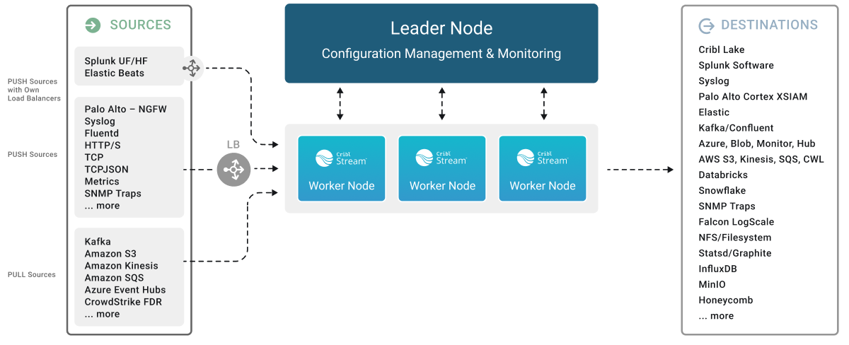
The main thing to consider with multiple Workers is that you’ll need a load balancer for all Push Sources that don’t natively support balancing across multiple Worker Nodes. You can see this added load balancer called out (as LB) in our Distributed Deployment Architecture diagram:
How Many Worker Nodes?
The next consideration is, how many Worker Nodes do you need? Having multiple Worker Nodes allows you to continue processing data while one Node is down for maintenance - so your sizing is determined by the remaining Worker Nodes. Here, you have a matrix of adjusting scaling vertically vs. horizontally, so let’s look at the math:
Effectively, 2 Worker Nodes means you lose 50% capacity when one is down. With 3 Nodes, you lose 33%. With 6 Nodes, you lose 17%. You will lose 2 vCPUs in overhead on each Node, but at larger scales, the benefits outweigh the costs.
Let’s look at an example using the naive 400GB/day per core capacity (i.e., 200GB/day per vCPU or Worker Process). We’ll pick approximately comparable desired throughput of 5.6-6TB/day, and see how the math works out.
2 Worker Nodes
32 vCPUs x2 Nodes = 64 vCPUs (- 2 vCPUs/Node for overhead) = 60 WPs
1 Node downs during patching: 30 WPs*0.2=6 TB capacity
6 TB/64 vCPUs = 0.09 TB/vCPU
3 Worker Nodes
16 vCPUs x3 Nodes = 48 vCPUs (-2 vCPUs/Node for overhead) = 42 WPs
1 Node downs during patching: 28 WPs*0.2=5.6 TB capacity
5.6 TB/48 vCPUs = 0.12 TB/vCPU
6 Worker Nodes
8 vCPUs x6 = 48 vCPUs (-2 vCPUs/Node for overhead) = 36 WPs
1 Node downs during patching: 30 WPs*0.2 TB/WP = 6 TB capacity
6TB/40 vCPUs = 0.15 TB/vCPU
As we can see, once your required throughput is high enough to make the 2 vCPU/Node tax negligible, a larger number of Worker Nodes is advantageous. You can do the math for your specific use case - remembering to adjust for expected peak usage and desired spike tolerance.
That said, having 3 Worker Nodes is usually the recommended minimum, since this provides resilience against unplanned outages even when one Worker is down for planned maintenance.
Where a Single Worker Group Can Fail
Even provisioning an “adequate” number of Worker Nodes, in a single Worker Group, might not be fully resilient if you encounter connection pinning, data bursts, or other unexpected resource demands.
Pinning
In Single-Instance Deployment above, we included the caveat of “assuming that the load is distributed evenly among all Worker Processes.” In reality, you need to validate this assumption. In some situations, you’ll need to take additional measures to assure that it’s true, or work around cases when it is not.
Pinning is a situation where a single TCP or UDP Source is sending a large amount of data over a single connection, causing that connection to be “pinned” to a single Worker Process. If the throughput is high enough, and the load balancer is unable to break up that connection, the affected Worker Processes might be overloaded and unable to keep up.
In a Distributed Deployment, to mitigate pinning, the Syslog Source provides a TCP Load Balancing option, as do the TCP JSON and Cribl TCP Sources.
On TCP Sources and deployments where these options are unavailable, you can minimize pinning by having the sender establish separate connections. If that’s not possible, try isolating a Worker Group that receives this input from all other processing responsibilities - this will maximize the throughput that this Group can handle.
Burst Loads Affecting Push Sources
Most of the time, your Push Sources will generate a reasonably predictable, consistent load. Using the sizing considerations outlined above, you should be able to come up with a Worker Group sized appropriately for your desired risk-versus-cost balance.
However, this balance can be upset when you have a surge of data that makes your system temporarily busier than you accounted for. The greatest impact would be felt by Push Sources that have no way to handle backpressure, such as UDP Sources.
A prime example of data burst is an ad-hoc run of a large Collection job. With multiple Worker Groups, you can separate Push versus Pull Sources, and can even use an Auto Scaling group group for large Collection jobs if desired.
Unexpected Resource Hogs
Our throughput estimates are based on certain assumptions about the average level of complexity of operations performed on the data. As you’re creating your Pipelines, at some point you might decide that you require additional resources to meet your data-processing needs. Certain combinations of Function, logic, and throughput will consume extra resources.
When expanded resource demands happen in a predictable, controlled manner, all is well. However, we’ve seen cases where an inefficient regular expression, or a memory-hungry custom Collection script, will cause a whole Worker Group to get overloaded. This leads to crashes, or to performance poor enough to cause data loss. Pipeline profiling helps with some of this. But using separate Worker Groups is an option to provide additional isolation.
Multiple Worker Groups
At the beginning of Distributed Deployment, we considered the limitations of a single Worker Group, and examined some strictly sizing-related reasons for multiple Worker Groups. Here, let’s consider some other reasons you might decide to take advantage of multiple Worker Groups.
In some cases, it makes sense to create separate Worker Groups, each close to their data. In other cases, multiple Groups might be necessary for your architecture based on other needs. Here are a few examples, which might not be directly applicable to your scenario, but which should help you realize when multiple Groups might benefit your deployment:
- Keeping Workers close to their data to optimize syslog over UDP.
- Controlling egress costs, by reducing and compressing data before it leaves your cloud provider’s region.
- Separating Push Sources versus Pull/Collector Sources.
- Geographical restrictions on data location, such as GDPR.
- Reducing or increasing the number of Workers connecting with a Source or a Destination.
- Centralize certain processing that is dependent on external systems, such as Redis lookups.
- Reducing the frequency of Stream config deployments, in cases where a deployment might disrupt data flow - such as triggering rebalancing among Kafka-based Sources.
Conclusion
As you can see by now, our “it depends” subtitle applies. But we hope that reading this guide has familiarized you with key aspects of what “it” depends on. There is no single “best practice” for sizing, because your own best architecture will depend on considering all options, including your risk-versus-cost balance, to define your own solution.
Equipped with the contents of this guide, you should be able to make better decisions about the potential risks and mitigations appropriate for your environment. After initial deployment, you can monitor utilization trends in the different resources we covered. As your needs evolve, so can your architecture. You’ll make assumptions, and when the potential for failure is beyond your tolerance, you can adjust accordingly.
Some final considerations: Is it worth stress-testing your environment, or a downscaled version of it? What’s the likelihood of everything going wrong at the same time - your throughput volume spiking to the highest acceptable level, while your Destinations are unavailable and your Persistent Queues are filling up? It depends.
To firm up your own architecture, consult Cribl support, Community Slack, or the Cribl Solutions Engineering or Professional Services experts dedicated to your deployment.